本文翻译自 Hugging Face 博客：https://huggingface.co/blog/annotated-diffusion

在这篇文章，我们深入了解降噪扩散模型（Denoising Diffusion Probabilistic Models）（也称作 DDPMs，diffusion models，score-based generative models 或者只简单地叫做 autoencoders）。研究者们已经可以在有条件或无条件的情况下生成图像/视频/语音。流行的例子包括 OpenAI 的 GLIDE、University of Heidelberg 的Latent Diffusion、Google Brain 的ImageGen。

我们将重温原始的 DDPM 论文 (Ho et al., 2020)，一步一步用 pytorch 实现（基于 Phil Wang 的代码实现，原始版本是tensorflow实现的）。注意，扩散的思想用于生成模型早在 (Sohl-Dickstein et al., 2015)中就被介绍了。但是，直到 (Song et al., 2019，斯坦福大学) 然后是 (Ho et al., 2020，Google Brain)才独立改进了此方法。

注意，存在几种关于扩散模型的观点。这里我们采用离散时间（隐变量模型）的观点，但也一定要看看其他观点。

好了，让我们开始！

from IPython.display import Image
Image(filename='assets/78_annotated-diffusion/ddpm_paper.png')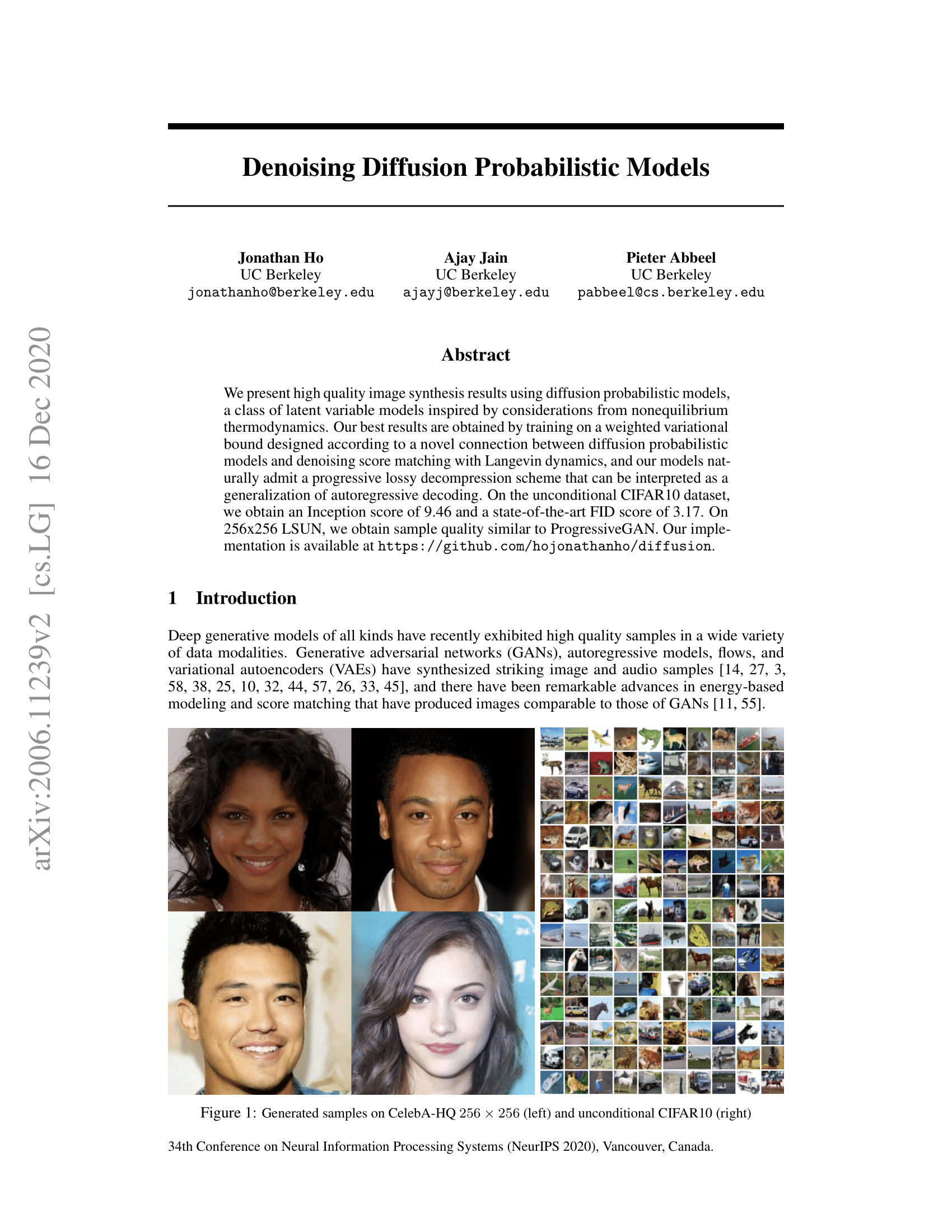

我们将导入所需要的包（假设你已经安装了 pytorch）。

!pip install -q -U einops datasets matplotlib tqdm

import math
from inspect import isfunction
from functools import partial

%matplotlib inline
import matplotlib.pyplot as plt
from tqdm.auto import tqdm
from einops import rearrange

import torch
from torch import nn, einsum
import torch.nn.functional as F

什么是扩散模型

（降噪）扩散模型相比于其他生成模型并不复杂，比如 Normalizing Flows、GANs、VAEs，它们都是将某个简单分布的噪声转为数据样本。也就是说，神经网络从纯噪声开始学习逐渐地降噪数据。

关于图像的更多细节，包括2个过程：

• 一个我们选择的固定的（或预设的）前向扩散过程$q$，它逐渐向图像添加高斯噪声，直到得到纯噪声。
• 一个学习得到的反向降噪扩散过程$p_\theta$，在这个过程中训练神经网络以降噪图像，从纯噪声开始直到真是图像。

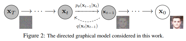
前向和反向过程都由发生在有限长时间步 $T$ 内的时间点 $t$ 来索引（DDPM作者使用 $T=1000$）。你从 $t=0$ 开始，从你的数据分布中采样一个真实图像 ${\bf x}_0$，前向过程在每个时间点$t$从高斯分布中采样噪声，这些噪声加到前一个时间步的图像中。给定一个足够大的$T$和一个在每个时间步中添加噪声的良好的schedule，你就会通过一个渐进的过程得到$t=T$处各向同性的高斯分布。

更加数学的形式

让我们更正式地写下来，因为最终我们需要一个易于处理的损失函数。

让 $q({\bf x}_0)$ 为真实数据分布，我们从这个分布采样得到图像，${\bf x}_0 \sim q({\bf x}_0)$。我们定义前向扩散过程 $q(\bf{x}_t | \bf{x}_{t-1})$，在每个时间步增加$t$增加高斯噪声，根据一个已知的变量 schdule $0<\beta_1<\beta_2< \dots < \beta_{T}<1$，即：

$$
q({\bf x}_t | {\bf x}_{t-1}) = \mathcal N({\bf x}_t; \sqrt{1-\beta_t} {\bf x}_{t-1}, \beta_t {\bf I})
$$

回忆一下，一个正太分布（也叫做高斯分布）被两个参数定义：均值 $\mu$ 和方差 $\sigma^2 \geq 0$。每个在时间步 $t$ 的新图片（有点噪声）是从条件高斯分布生成的，参数为 $\mu_t = \sqrt{1-\beta_t} {\bf x}_t$ 和 $\sigma_t^2 = \beta_t$，我们可以从 $\epsilon \sim \mathcal N (\bf{0}, \bf{I})$ 中采样，然后设 ${\bf x}_t = \sqrt{1 – \beta_t} {\bf x}_{t-1} + \sqrt{\beta_t} \epsilon$。

注意 $\beta_t$ 在每个时间步不是常数（带了时间 $t$ 下标），事实上我们定义了一个所谓的“方差 schedule”，它可以是线性的、二次方的、余弦的等等，我们将进一步看到（有点像学习率 schedule）。

从 ${\bf x}_0$ 开始，最终得到 ${\bf x}_1, \dots, {\bf x}_t, \dots, {\bf x}_T$，如果我们合理地设置 schedule，${\bf x}_T$ 就是纯高斯噪声。

现在，如果我们知道条件分布 $p({\bf x}_{t-1} | {\bf x}_t)$，我们可以反省运行这个过程：通过采样一些随机高斯噪声 ${\bf x}_T$，逐渐降噪它，这样我们就可以从真实分布 ${\bf x}_0$ 中得到一个样本。

然而，我们不知道 $p({\bf x}_{t-1} | {\bf x}_t)$。这很棘手，因为它需要知道所有可能图像的分布才能计算这个条件概率。 因此，我们将利用神经网络来近似（学习）这个条件概率分布，我们称为 $p_{\theta}({\bf x}_{t-1} | {\bf x}_t)$，$\theta$ 为神经网络的参数，根据梯度下降来更新。

所以我们需要一个神经网络来表示后向过程的（条件）概率分布。 如果我们假设这个逆向过程也是高斯分布，那么回想一下任何高斯分布都由 2 个参数定义：

• 由 $\mu_{\theta}$ 参数化的均值；
• 由 $\Sigma_{\theta}$ 参数化的方差；

因此我们参数化这个过程为：

$$
p_{\theta} ({\bf x}_{t-1} | {\bf x}_t) = \mathcal N ({\bf x}_{t-1}; \mu_{\theta}({\bf x}_t, t), \Sigma_{\theta}({\bf x}_t, t))
$$

其中均值和方差也以噪声水平 $t$ 为条件。

因此，我们的神经网络需要学习/表示均值和方差。然而，DDPM 作者决定保持方差固定，让神经网络只学习（表示）这个条件概率分布的均值 $\mu_{\theta}$。来自论文：

首先，我们设 $\Sigma_{\theta}({\bf x}_t, t) = \sigma_t^2 {\bf I}$ 为未经训练的时间相关常数。从经验上来看，$\sigma_t^2=\beta_t$ 和 $\sigma_t^2 = \tilde{\beta_t}$ （见论文）有相似的结果。

后来在改进的扩散模型论文中对此进行了改进，其中神经网络除了均值之外还学习了这个向后过程的方差。

继续，假设我们的神经网络只需要学习/表示条件概率分布的均值。

定义一个目标函数（通过表示均值）

为了推导出学习后向过程均值的目标函数，作者观察到 $q$ 和 $p_{\theta}$ 的结合可以看作变分自编码器（VAE）（Kingma et al., 2013）。因此，变分下界（也称为 ELBO）可用于最小化关于真实数据样本 ${\bf x}_0$ 的负对数似然（有关 ELBO 的详细信息，我们参考 VAE 论文）。事实证明，这个过程的 ELBO 是每个时间步的损失总和，$L = L_0 + L_1 + \dots + L_T$。通过前向 $q$ 过程和后向过程的构造，损失的每一项（除了 $L_0$）实际上是2个高斯分布之间的KL散度，可以明确地写成关于均值的L2-损失！

如 Sohl-Dickstein 等人所示，构造正向过程 $q$ 的直接结果是我们可以在以 ${\bf x}_0$ 为条件的任意噪声水平下对 $\bf x$ 进行采样（因为高斯和也是高斯）。这很方便，我们不需要为了采样 ${\bf x}_0$ 重复地应用 $q$。我们有：

$$
q({\bf x}_t | {\bf x}_0) = \mathcal N ({\bf x}_t; \sqrt{\bar{\alpha_t}}{\bf x}_0, (1-\bar{\alpha_t}){\bf I})
$$

其中 $\alpha_t := 1-\beta_t$，$\bar{\alpha_t} := \prod_{s=1}^{t} \alpha_s$。让我们将这个等式称为 “nice property”。这意味着我们可以对高斯噪声进行采样并适当地缩放它，把它直接加给 ${\bf x}_0$ 得到 ${\bf x}_t$。请注意，$\bar{\alpha_t}$ 是已知 $\beta_t$ 方差 schedule 的函数，因此也是已知的并且可以预先计算。这允许我们在训练过程中可以优化损失函数 $L$ 的随机项（也就是说，在训练过程中随机采样 $t$ 并优化 $L_t$）。

如 Ho 等人所示，此属性的另一个优点是可以（经过一些数学运算，为此我们建议读者阅读这篇优秀的博客文章）不重新参数化均值以使神经网络学习（预测）（通过网络 $\epsilon_{\theta}({\bf x}_t, t)$）构成损失的 KL 项中噪声水平 $t$ 的附加噪声。这意味着我们的神经网络变成了一个噪声预测器，而不是直接的均值预测器。均值可以由下式计算：

$$
\mu_\theta\left(\mathbf{x}_t, t\right)=\frac{1}{\sqrt{\alpha_t}}\left(\mathbf{x}_t-\frac{\beta_t}{\sqrt{1-\bar{\alpha}_t}} \epsilon_\theta\left(\mathbf{x}_t, t\right)\right)
$$

最终的损失函数 $L_t$ （对于给定 $\epsilon \sim \mathcal N(\bf 0, I)$ 下一个随机时间步 $t$）为：

$$
\left\lVert \epsilon – \epsilon_\theta (\mathbf{x}_t, t) \right\rVert ^2= \left\lVert \epsilon – \epsilon_\theta (\sqrt{\bar{\alpha}_t} \mathbf{x}_0+\sqrt{ (1-\bar{\alpha}_t )} \epsilon, t ) \right\rVert ^2
$$

这里 ${\bf x}_0$ 是初始（真实的未被破坏的）图像，我们看到固定前向过程给出的直接噪声水平 $t$ 样本。$\epsilon$ 是在时间步 $t$ 采样的纯噪声，$\epsilon_{\theta}({\bf x}_t, t)$ 是我们的神经网络。神经网络使用真实和预测高斯噪声之间的简单均方误差 (MSE) 进行优化。

那么现在的训练算法为：

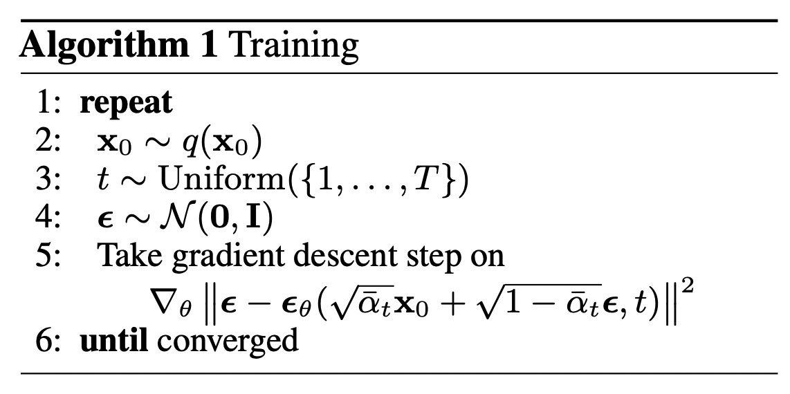
也就是说：

• 我们从真实未知的可能复杂的数据分布 $q({\bf x}_0)$ 中随机采样 ${\bf x}_0$
• 在1和 $T$ 之间均匀地采样噪声水平 $t$（也就是随机时间步）
• 从高斯噪声中随机采样噪声，通过这个在水平 $t$ 的噪声破坏输入（利用上面定义的 nice property）
• 基于被破坏的图像 ${\bf x}_t$（也就是基于已知的 schedule $\beta_t$ 在 ${\bf x}_0$ 上应用噪声）训练神经网络以预测这个噪声

实际上，所有这些都是在批量数据上完成的，因为人们使用随机梯度下降来优化神经网络。

神经网络

神经网络需要在特定时间步长处接收噪声图像并返回预测噪声。 请注意，预测噪声是与输入图像具有相同大小/分辨率的张量。 所以从技术上讲，网络接收和输出相同形状的张量。 我们可以为此使用哪种类型的神经网络？

这里通常使用的与自动编码器非常相似，你去可能还记得典型的“深度学习入门”教程。 自动编码器在编码器和解码器之间有一个所谓的“bottleneck”层。 编码器首先将图像编码成称为“bottleneck”的较小隐藏表示，然后解码器将该隐藏表示解码回实际图像。 这迫使网络只在瓶颈层保留最重要的信息。

在架构方面，DDPM 作者选择了由 (Ronneberger et al., 2015) 引入的 U-Net（当时，它在医学图像分割方面取得了最先进的结果）。 这个网络，像任何自动编码器一样，中间有一个瓶颈，确保网络只学习最重要的信息。 重要的是，它在编码器和解码器之间引入了残差连接，极大地改善了梯度流（受 He et al., 2015 中的 ResNet 启发）。

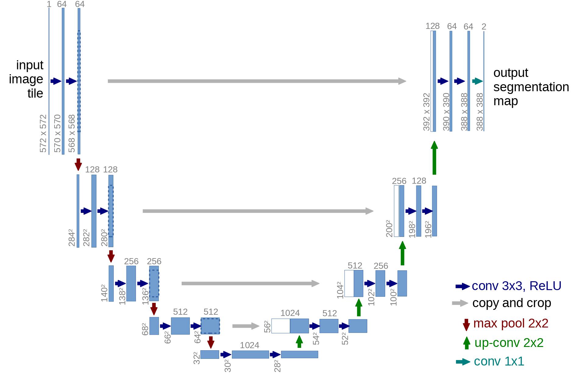
可以看出，U-Net 模型首先对输入进行下采样（即使输入在空间分辨率方面更小），然后进行上采样。

下面，我们逐步实现这个网络。

Network helpers

首先，我们定义了一些辅助函数和类，它们将在实现神经网络时使用。 重要的是，我们定义了一个残差模块，它只是将输入添加到特定函数的输出（换句话说，将残差连接添加到特定函数）。

我们还为上采样和下采样操作定义了别名。

def exists(x):
    return x is not None

def default(val, d):
    if exists(val):
        return val
    return d() if isfunction(d) else d

def num_to_groups(num, divisor):
    groups = num // divisor
    remainder = num % divisor
    arr = [divisor] * groups
    if remainder > 0:
        arr.append(remainder)
    return arr

class Residual(nn.Module):
    def __init__(self, fn):
        super().__init__()
        self.fn = fn

    def forward(self, x, *args, **kwargs):
        return self.fn(x, *args, **kwargs) + x

def Upsample(dim, dim_out=None):
    return nn.Sequential(
        nn.Upsample(scale_factor=2, mode="nearest"),
        nn.Conv2d(dim, default(dim_out, dim), 3, padding=1),
    )

def Downsample(dim, dim_out=None):
    # No More Strided Convolutions or Pooling
    return nn.Sequential(
        Rearrange("b c (h p1) (w p2) -> b (c p1 p2) h w", p1=2, p2=2),
        nn.Conv2d(dim * 4, default(dim_out, dim), 1),
    )

Position embeddings

由于神经网络的参数跨时间共享（噪声水平），作者受 Transformer 的启发，采用正弦位置嵌入对 $t$ 进行编码（Vaswani 等人，2017 年）。 这使得神经网络“知道”它在哪个特定时间步长（噪声水平）运行，对于批次中的每个图像。

SinusoidalPositionEmbeddings 模块将形状为 (batch_size, 1) 的张量作为输入（即一批中几个噪声图像的噪声水平），并将其转换为形状为 (batch_size, dim) 的张量，其中 dim 是图位置嵌入的维数。 然后将其添加到每个残差块中，我们将进一步看到。

class SinusoidalPositionEmbeddings(nn.Module):
    def __init__(self, dim):
        super().__init__()
        self.dim = dim

    def forward(self, time):
        device = time.device
        half_dim = self.dim // 2
        embeddings = math.log(10000) / (half_dim - 1)
        embeddings = torch.exp(torch.arange(half_dim, device=device) * -embeddings)
        embeddings = time[:, None] * embeddings[None, :]
        embeddings = torch.cat((embeddings.sin(), embeddings.cos()), dim=-1)
        return embeddings

ResNet block

接下来，我们定义 U-Net 模型的核心构建块。 DDPM 作者采用了 Wide ResNet 块（Zagoruyko et al., 2016），但 Phil Wang 已将标准卷积层替换为“权重标准化”版本，该版本与 group normalization 结合使用效果更好（参见（Kolesnikov et al., 2019）了解详情）。

class WeightStandardizedConv2d(nn.Conv2d):
    """
    https://arxiv.org/abs/1903.10520
    weight standardization purportedly works synergistically with group normalization
    """

    def forward(self, x):
        eps = 1e-5 if x.dtype == torch.float32 else 1e-3

        weight = self.weight
        mean = reduce(weight, "o ... -> o 1 1 1", "mean")
        var = reduce(weight, "o ... -> o 1 1 1", partial(torch.var, unbiased=False))
        normalized_weight = (weight - mean) * (var + eps).rsqrt()

        return F.conv2d(
            x,
            normalized_weight,
            self.bias,
            self.stride,
            self.padding,
            self.dilation,
            self.groups,
        )

class Block(nn.Module):
    def __init__(self, dim, dim_out, groups=8):
        super().__init__()
        self.proj = WeightStandardizedConv2d(dim, dim_out, 3, padding=1)
        self.norm = nn.GroupNorm(groups, dim_out)
        self.act = nn.SiLU()

    def forward(self, x, scale_shift=None):
        x = self.proj(x)
        x = self.norm(x)

        if exists(scale_shift):
            scale, shift = scale_shift
            x = x * (scale + 1) + shift

        x = self.act(x)
        return x

class ResnetBlock(nn.Module):
    """https://arxiv.org/abs/1512.03385"""

    def __init__(self, dim, dim_out, *, time_emb_dim=None, groups=8):
        super().__init__()
        self.mlp = (
            nn.Sequential(nn.SiLU(), nn.Linear(time_emb_dim, dim_out * 2))
            if exists(time_emb_dim)
            else None
        )

        self.block1 = Block(dim, dim_out, groups=groups)
        self.block2 = Block(dim_out, dim_out, groups=groups)
        self.res_conv = nn.Conv2d(dim, dim_out, 1) if dim != dim_out else nn.Identity()

    def forward(self, x, time_emb=None):
        scale_shift = None
        if exists(self.mlp) and exists(time_emb):
            time_emb = self.mlp(time_emb)
            time_emb = rearrange(time_emb, "b c -> b c 1 1")
            scale_shift = time_emb.chunk(2, dim=1)

        h = self.block1(x, scale_shift=scale_shift)
        h = self.block2(h)
        return h + self.res_conv(x)

Attention module

接下来，我们定义注意力模块，DDPM 作者将其添加到卷积块之间。 注意力是著名的 Transformer 架构的基石（Vaswani et al., 2017），它在 AI 的各个领域都取得了巨大的成功，从 NLP 和视觉到蛋白质折叠。 Phil Wang 使用了两种注意力变体：一种是常规的多头自注意力（在 Transformer 中使用），另一种是线性注意力变体（Shen et al., 2018），其时间和内存需求与序列长度成线性比例，这和常规注意力的二次方相反。

对于注意力机制的扩展解释，我们建议读者阅读 Jay Allamar 的精彩博客文章。

class Attention(nn.Module):
    def __init__(self, dim, heads=4, dim_head=32):
        super().__init__()
        self.scale = dim_head**-0.5
        self.heads = heads
        hidden_dim = dim_head * heads
        self.to_qkv = nn.Conv2d(dim, hidden_dim * 3, 1, bias=False)
        self.to_out = nn.Conv2d(hidden_dim, dim, 1)

    def forward(self, x):
        b, c, h, w = x.shape
        qkv = self.to_qkv(x).chunk(3, dim=1)
        q, k, v = map(
            lambda t: rearrange(t, "b (h c) x y -> b h c (x y)", h=self.heads), qkv
        )
        q = q * self.scale

        sim = einsum("b h d i, b h d j -> b h i j", q, k)
        sim = sim - sim.amax(dim=-1, keepdim=True).detach()
        attn = sim.softmax(dim=-1)

        out = einsum("b h i j, b h d j -> b h i d", attn, v)
        out = rearrange(out, "b h (x y) d -> b (h d) x y", x=h, y=w)
        return self.to_out(out)

class LinearAttention(nn.Module):
    def __init__(self, dim, heads=4, dim_head=32):
        super().__init__()
        self.scale = dim_head**-0.5
        self.heads = heads
        hidden_dim = dim_head * heads
        self.to_qkv = nn.Conv2d(dim, hidden_dim * 3, 1, bias=False)

        self.to_out = nn.Sequential(nn.Conv2d(hidden_dim, dim, 1), 
                                    nn.GroupNorm(1, dim))

    def forward(self, x):
        b, c, h, w = x.shape
        qkv = self.to_qkv(x).chunk(3, dim=1)
        q, k, v = map(
            lambda t: rearrange(t, "b (h c) x y -> b h c (x y)", h=self.heads), qkv
        )

        q = q.softmax(dim=-2)
        k = k.softmax(dim=-1)

        q = q * self.scale
        context = torch.einsum("b h d n, b h e n -> b h d e", k, v)

        out = torch.einsum("b h d e, b h d n -> b h e n", context, q)
        out = rearrange(out, "b h c (x y) -> b (h c) x y", h=self.heads, x=h, y=w)
        return self.to_out(out)

Group normalization

DDPM 作者将 U-Net 的卷积层/注意力层与 group normalization 交织在一起（Wu et al., 2018）。 下面，我们定义了一个 PreNorm 类，它将用于在注意力层之前应用 groupnorm。 请注意，关于在 Transformers 应该在注意力之前还是之后添加 normalization 一直存在争议。

class PreNorm(nn.Module):
    def __init__(self, dim, fn):
        super().__init__()
        self.fn = fn
        self.norm = nn.GroupNorm(1, dim)

    def forward(self, x):
        x = self.norm(x)
        return self.fn(x)

条件 U-Net

现在我们已经定义了所有构建块（position embeddings、ResNet blocks、attention 和 group normalization），是时候去定义整个网络了。会议一下网络 $\epsilon_{\theta}({\bf x}_t, t)$的任务是把一批有噪声的图像和它们各自的噪声水平都拿进来，然后输出噪声，这个噪声是添加到图片里的噪声。也就是：

• 神经网络拿形状为(batch_size, num_channels, height, width) 的噪声图片和形状为 (batch_size 1) 的噪声水平作为输入，然后返回一个形状为 (batch_size, num_channels, height, width) 的张量。

网络构建如下：

• 首先，一个卷积层应用在一批噪声图像上，并且为噪声水平计算位置编码
• 然后，应用一系列的下采样阶段。每个下采样阶段包括两个 ResNet 块 + groupnorm + attention + residual connection + 一个下采样操作
• 在网络的中间，再次应用 ResNet 块，与注意力交错
• 接下来，应用一系列的上采样阶段。每个上采样阶段包括两个 ResNet 块 + groupnorm + attention + residual connection + 一个上采样操作
• 最后，应用了一个 ResNet 块和一个卷积层。

最终，神经网络层层叠叠，就好像它们是乐高积木一样（但了解它们的工作原理很重要）。

class Unet(nn.Module):
    def __init__(
        self,
        dim,
        init_dim=None,
        out_dim=None,
        dim_mults=(1, 2, 4, 8),
        channels=3,
        self_condition=False,
        resnet_block_groups=4,
    ):
        super().__init__()

        # determine dimensions
        self.channels = channels
        self.self_condition = self_condition
        input_channels = channels * (2 if self_condition else 1)

        init_dim = default(init_dim, dim)
        self.init_conv = nn.Conv2d(input_channels, init_dim, 1, padding=0) # changed to 1 and 0 from 7,3

        dims = [init_dim, *map(lambda m: dim * m, dim_mults)]
        in_out = list(zip(dims[:-1], dims[1:]))

        block_klass = partial(ResnetBlock, groups=resnet_block_groups)

        # time embeddings
        time_dim = dim * 4

        self.time_mlp = nn.Sequential(
            SinusoidalPositionEmbeddings(dim),
            nn.Linear(dim, time_dim),
            nn.GELU(),
            nn.Linear(time_dim, time_dim),
        )

        # layers
        self.downs = nn.ModuleList([])
        self.ups = nn.ModuleList([])
        num_resolutions = len(in_out)

        for ind, (dim_in, dim_out) in enumerate(in_out):
            is_last = ind >= (num_resolutions - 1)

            self.downs.append(
                nn.ModuleList(
                    [
                        block_klass(dim_in, dim_in, time_emb_dim=time_dim),
                        block_klass(dim_in, dim_in, time_emb_dim=time_dim),
                        Residual(PreNorm(dim_in, LinearAttention(dim_in))),
                        Downsample(dim_in, dim_out)
                        if not is_last
                        else nn.Conv2d(dim_in, dim_out, 3, padding=1),
                    ]
                )
            )

        mid_dim = dims[-1]
        self.mid_block1 = block_klass(mid_dim, mid_dim, time_emb_dim=time_dim)
        self.mid_attn = Residual(PreNorm(mid_dim, Attention(mid_dim)))
        self.mid_block2 = block_klass(mid_dim, mid_dim, time_emb_dim=time_dim)

        for ind, (dim_in, dim_out) in enumerate(reversed(in_out)):
            is_last = ind == (len(in_out) - 1)

            self.ups.append(
                nn.ModuleList(
                    [
                        block_klass(dim_out + dim_in, dim_out, time_emb_dim=time_dim),
                        block_klass(dim_out + dim_in, dim_out, time_emb_dim=time_dim),
                        Residual(PreNorm(dim_out, LinearAttention(dim_out))),
                        Upsample(dim_out, dim_in)
                        if not is_last
                        else nn.Conv2d(dim_out, dim_in, 3, padding=1),
                    ]
                )
            )

        self.out_dim = default(out_dim, channels)

        self.final_res_block = block_klass(dim * 2, dim, time_emb_dim=time_dim)
        self.final_conv = nn.Conv2d(dim, self.out_dim, 1)

    def forward(self, x, time, x_self_cond=None):
        if self.self_condition:
            x_self_cond = default(x_self_cond, lambda: torch.zeros_like(x))
            x = torch.cat((x_self_cond, x), dim=1)

        x = self.init_conv(x)
        r = x.clone()

        t = self.time_mlp(time)

        h = []

        for block1, block2, attn, downsample in self.downs:
            x = block1(x, t)
            h.append(x)

            x = block2(x, t)
            x = attn(x)
            h.append(x)

            x = downsample(x)

        x = self.mid_block1(x, t)
        x = self.mid_attn(x)
        x = self.mid_block2(x, t)

        for block1, block2, attn, upsample in self.ups:
            x = torch.cat((x, h.pop()), dim=1)
            x = block1(x, t)

            x = torch.cat((x, h.pop()), dim=1)
            x = block2(x, t)
            x = attn(x)

            x = upsample(x)

        x = torch.cat((x, r), dim=1)

        x = self.final_res_block(x, t)
        return self.final_conv(x)

定义前向扩散过程

前向扩散过程在多个时间步长 $T$ 中逐渐给一张来自真实分布的图像增加噪声。这是根据方差 schedule 发生的。原始的 DDPM 采用了线性 schedule：

我们将前向过程方差设为线性增长，从 $\beta_1 = 10^{-4}$ 到 $\beta_T = 0.02$。

然而，（Nichol et al., 2021）表明采用 余弦 schedule 能达到更好的结果。

下面我们为时间步长 $T$ 定义方差 schedule（后面我们会选择一个）。

def cosine_beta_schedule(timesteps, s=0.008):
    """
    cosine schedule as proposed in https://arxiv.org/abs/2102.09672
    """
    steps = timesteps + 1
    x = torch.linspace(0, timesteps, steps)
    alphas_cumprod = torch.cos(((x / timesteps) + s) / (1 + s) * torch.pi * 0.5) ** 2
    alphas_cumprod = alphas_cumprod / alphas_cumprod[0]
    betas = 1 - (alphas_cumprod[1:] / alphas_cumprod[:-1])
    return torch.clip(betas, 0.0001, 0.9999)

def linear_beta_schedule(timesteps):
    beta_start = 0.0001
    beta_end = 0.02
    return torch.linspace(beta_start, beta_end, timesteps)

def quadratic_beta_schedule(timesteps):
    beta_start = 0.0001
    beta_end = 0.02
    return torch.linspace(beta_start**0.5, beta_end**0.5, timesteps) ** 2

def sigmoid_beta_schedule(timesteps):
    beta_start = 0.0001
    beta_end = 0.02
    betas = torch.linspace(-6, 6, timesteps)
    return torch.sigmoid(betas) * (beta_end - beta_start) + beta_start

首先，我们为 $T=300$ 时间步长使用线性 schedule，并根据我们需要的 $\beta_t$ 定义各种变量，例如方差 $\bar{\alpha}_t$ 的累计乘积。下面的每个变量都是一维张量，存储从 $t$ 到 $T$ 的值。重要的是，我们还定义了一个 extract 函数，它将允许我们为一批索引提取适当的 $t$ 索引。

我们将用一张猫的图像来说明在扩散过程中每个时间步的噪声是如何添加的。

from PIL import Image
import requests

url = 'http://images.cocodataset.org/val2017/000000039769.jpg'
image = Image.open(requests.get(url, stream=True).raw)
image

噪声被添加到 PyTorch 张量，而不是 Pillow Images。 我们将首先定义图像转换，使我们能够从 PIL 图像转换为 PyTorch 张量（我们可以在其上添加噪声），反之亦然。

这些变换是很简单的：我们首先同通过除以255将图像归一化（这样它们在 $[0, 1]$ 范围内），然后保证它们在 $[-1, 1]$ 范围内。来自 DDPM 论文：

我们假设图像数据由 ${0, 1, \dots, 255}$ 的整数组成，被缩放到 $[-1, 1]$。这确保了神经网络逆向过程从标准正态先验 $p({\bf x}_T)$ 开始对一致缩放的输入进行操作。

from torchvision.transforms import Compose, ToTensor, Lambda, ToPILImage, CenterCrop, Resize

image_size = 128
transform = Compose([
    Resize(image_size),
    CenterCrop(image_size),
    ToTensor(), # turn into Numpy array of shape HWC, divide by 255
    Lambda(lambda t: (t * 2) - 1),

])

x_start = transform(image).unsqueeze(0)
x_start.shape

Output:
----------------------------------------------------------------------------------------------------
torch.Size([1, 3, 128, 128])

我们还定义了逆向变换，它接收一个值在 $[-1, 1]$ 之间的 PyTorch 张量，并转为 PIL 张量：

import numpy as np

reverse_transform = Compose([
     Lambda(lambda t: (t + 1) / 2),
     Lambda(lambda t: t.permute(1, 2, 0)), # CHW to HWC
     Lambda(lambda t: t * 255.),
     Lambda(lambda t: t.numpy().astype(np.uint8)),
     ToPILImage(),
])

让我们验证一下：

reverse_transform(x_start.squeeze())

现在我们可以定义论文里的前向扩散过程了：

# forward diffusion (using the nice property)
def q_sample(x_start, t, noise=None):
    if noise is None:
        noise = torch.randn_like(x_start)

    sqrt_alphas_cumprod_t = extract(sqrt_alphas_cumprod, t, x_start.shape)
    sqrt_one_minus_alphas_cumprod_t = extract(
        sqrt_one_minus_alphas_cumprod, t, x_start.shape
    )

    return sqrt_alphas_cumprod_t * x_start + sqrt_one_minus_alphas_cumprod_t * noise

让我们在一个特定的时间步上测试：

def get_noisy_image(x_start, t):
  # add noise
  x_noisy = q_sample(x_start, t=t)

  # turn back into PIL image
  noisy_image = reverse_transform(x_noisy.squeeze())

  return noisy_image

# take time step
t = torch.tensor([40])

get_noisy_image(x_start, t)

让我们将其可视化为不同的时间步长：

import matplotlib.pyplot as plt

# use seed for reproducability
torch.manual_seed(0)

# source: https://pytorch.org/vision/stable/auto_examples/plot_transforms.html#sphx-glr-auto-examples-plot-transforms-py
def plot(imgs, with_orig=False, row_title=None, **imshow_kwargs):
    if not isinstance(imgs[0], list):
        # Make a 2d grid even if there's just 1 row
        imgs = [imgs]

    num_rows = len(imgs)
    num_cols = len(imgs[0]) + with_orig
    fig, axs = plt.subplots(figsize=(200,200), nrows=num_rows, ncols=num_cols, squeeze=False)
    for row_idx, row in enumerate(imgs):
        row = [image] + row if with_orig else row
        for col_idx, img in enumerate(row):
            ax = axs[row_idx, col_idx]
            ax.imshow(np.asarray(img), **imshow_kwargs)
            ax.set(xticklabels=[], yticklabels=[], xticks=[], yticks=[])

    if with_orig:
        axs[0, 0].set(title='Original image')
        axs[0, 0].title.set_size(8)
    if row_title is not None:
        for row_idx in range(num_rows):
            axs[row_idx, 0].set(ylabel=row_title[row_idx])

    plt.tight_layout()

plot([get_noisy_image(x_start, torch.tensor([t])) for t in [0, 50, 100, 150, 199]])

这意味着我们现在可以定义给定模型的损失函数，如下：

def p_losses(denoise_model, x_start, t, noise=None, loss_type="l1"):
    if noise is None:
        noise = torch.randn_like(x_start)

    x_noisy = q_sample(x_start=x_start, t=t, noise=noise)
    predicted_noise = denoise_model(x_noisy, t)

    if loss_type == 'l1':
        loss = F.l1_loss(noise, predicted_noise)
    elif loss_type == 'l2':
        loss = F.mse_loss(noise, predicted_noise)
    elif loss_type == "huber":
        loss = F.smooth_l1_loss(noise, predicted_noise)
    else:
        raise NotImplementedError()

    return loss

denoise_model 是我们在上面定义的 U-Net。我们在真实噪声和预测噪声之间采用 Huber 损失。

定义一个 PyTorch Dataset + DataLoader

这里我们定义一个常规的 Pytorch Dataset。数据集仅包括真实数据集中的图片，比如 Fashion-MNIST、CIFAR-10 或者 ImageNet，线性缩放到 $[-1, 1]$

每张图片被缩放到相同的尺寸。值得注意的是图片也进行了随机水平翻转。来自论文：

我们在 CIFAR10 的训练过程中使用了随机水平翻转； 我们尝试了使用翻转和不使用翻转的训练，发现翻转可以稍微提高样本质量。

这里我们使用 🤗 Datasets library 从 hub 中来加载 Fashion MNIST 数据集。这个数据集包含了已经是相同尺寸的图片，为 $28 \times 28$。

from datasets import load_dataset

# load dataset from the hub
dataset = load_dataset("fashion_mnist")
image_size = 28
channels = 1
batch_size = 128

接下来，我们定义一个函数，我们将在整个数据集上即时应用该函数。我们使用 with_transform 函数来实现。该函数仅应用一些基本的图像预处理：随机水平翻转、重新缩放并最终使它们在 $[-1, 1]$ 之间。

from torchvision import transforms
from torch.utils.data import DataLoader

# define image transformations (e.g. using torchvision)
transform = Compose([
            transforms.RandomHorizontalFlip(),
            transforms.ToTensor(),
            transforms.Lambda(lambda t: (t * 2) - 1)
])

# define function
def transforms(examples):
   examples["pixel_values"] = [transform(image.convert("L")) for image in examples["image"]]
   del examples["image"]

   return examples

transformed_dataset = dataset.with_transform(transforms).remove_columns("label")

# create dataloader
dataloader = DataLoader(transformed_dataset["train"], batch_size=batch_size, shuffle=True)

batch = next(iter(dataloader))
print(batch.keys())

Output:
----------------------------------------------------------------------------------------------------
dict_keys(['pixel_values'])

采样

由于我们将在训练期间从模型中采样（以便跟踪进度），因此我们在下面定义了代码。 采样在论文中总结为 Algorithm 2：

从扩散模型中生成新的图片通过反转扩散过程实现：我们从 $T$ 开始，这里我们从高斯分布中采样纯噪声，然后用我们的神经网络去逐渐地降噪它（用已经学习好的条件概率），直到在时间步 $t=0$ 结束。如上所示，我们可以推导出降噪程度稍差地图像 ${\bf x}_{t-1}$，通过使用我们的噪声预测器来插入均值的重新参数化。记住方差已经提前知道了。

理想情况下，结束时的图像开起来就像是来自真实分布的。

下面的代码实现了这个过程：

@torch.no_grad()
def p_sample(model, x, t, t_index):
    betas_t = extract(betas, t, x.shape)
    sqrt_one_minus_alphas_cumprod_t = extract(
        sqrt_one_minus_alphas_cumprod, t, x.shape
    )
    sqrt_recip_alphas_t = extract(sqrt_recip_alphas, t, x.shape)

    # Equation 11 in the paper
    # Use our model (noise predictor) to predict the mean
    model_mean = sqrt_recip_alphas_t * (
        x - betas_t * model(x, t) / sqrt_one_minus_alphas_cumprod_t
    )

    if t_index == 0:
        return model_mean
    else:
        posterior_variance_t = extract(posterior_variance, t, x.shape)
        noise = torch.randn_like(x)
        # Algorithm 2 line 4:
        return model_mean + torch.sqrt(posterior_variance_t) * noise 

# Algorithm 2 (including returning all images)
@torch.no_grad()
def p_sample_loop(model, shape):
    device = next(model.parameters()).device

    b = shape[0]
    # start from pure noise (for each example in the batch)
    img = torch.randn(shape, device=device)
    imgs = []

    for i in tqdm(reversed(range(0, timesteps)), desc='sampling loop time step', total=timesteps):
        img = p_sample(model, img, torch.full((b,), i, device=device, dtype=torch.long), i)
        imgs.append(img.cpu().numpy())
    return imgs

@torch.no_grad()
def sample(model, image_size, batch_size=16, channels=3):
    return p_sample_loop(model, shape=(batch_size, channels, image_size, image_size))

注意上面的代码是原始实现的简化版本。我们发现我们的简化（和论文的 Algorithm 2 一致）已经和原始实现工作得一样好，更复杂的实现 采用了 clipping。

训练模型

接下来，我们用常规的 PyTorch 风格训练模型。我们也定义了一些逻辑，用上面定义的sample 方法来周期性地保存生成的图片。

from pathlib import Path

def num_to_groups(num, divisor):
    groups = num // divisor
    remainder = num % divisor
    arr = [divisor] * groups
    if remainder > 0:
        arr.append(remainder)
    return arr

results_folder = Path("./results")
results_folder.mkdir(exist_ok = True)
save_and_sample_every = 1000

下面我们定义模型，将其放到 GPU。我们也定义了标准的优化器（Adam）。

from torch.optim import Adam

device = "cuda" if torch.cuda.is_available() else "cpu"

model = Unet(
    dim=image_size,
    channels=channels,
    dim_mults=(1, 2, 4,)
)
model.to(device)

optimizer = Adam(model.parameters(), lr=1e-3)

让我们开始训练！

from torchvision.utils import save_image

epochs = 6

for epoch in range(epochs):
    for step, batch in enumerate(dataloader):
      optimizer.zero_grad()

      batch_size = batch["pixel_values"].shape[0]
      batch = batch["pixel_values"].to(device)

      # Algorithm 1 line 3: sample t uniformally for every example in the batch
      t = torch.randint(0, timesteps, (batch_size,), device=device).long()

      loss = p_losses(model, batch, t, loss_type="huber")

      if step % 100 == 0:
        print("Loss:", loss.item())

      loss.backward()
      optimizer.step()

      # save generated images
      if step != 0 and step % save_and_sample_every == 0:
        milestone = step // save_and_sample_every
        batches = num_to_groups(4, batch_size)
        all_images_list = list(map(lambda n: sample(model, batch_size=n, channels=channels), batches))
        all_images = torch.cat(all_images_list, dim=0)
        all_images = (all_images + 1) * 0.5
        save_image(all_images, str(results_folder / f'sample-{milestone}.png'), nrow = 6)

Output:
----------------------------------------------------------------------------------------------------
Loss: 0.46477368474006653
Loss: 0.12143351882696152
Loss: 0.08106148988008499
Loss: 0.0801810547709465
Loss: 0.06122320517897606
Loss: 0.06310459971427917
Loss: 0.05681884288787842
Loss: 0.05729678273200989
Loss: 0.05497899278998375
Loss: 0.04439849033951759
Loss: 0.05415581166744232
Loss: 0.06020551547408104
Loss: 0.046830907464027405
Loss: 0.051029372960329056
Loss: 0.0478244312107563
Loss: 0.046767622232437134
Loss: 0.04305662214756012
Loss: 0.05216279625892639
Loss: 0.04748568311333656
Loss: 0.05107741802930832
Loss: 0.04588869959115982
Loss: 0.043014321476221085
Loss: 0.046371955424547195
Loss: 0.04952816292643547
Loss: 0.04472338408231735

采样（推理）

为了从模型中采样，我们使用上面定义的采样函数：

# sample 64 images
samples = sample(model, image_size=image_size, batch_size=64, channels=channels)

# show a random one
random_index = 5
plt.imshow(samples[-1][random_index].reshape(image_size, image_size, channels), cmap="gray")

看起来模型可以生成一个很好的 T-shirt 了！记住我们训练的数据集是低分辨率的（$28 \times 28$）。

我们也可以生成降噪过程的 gif：

import matplotlib.animation as animation

random_index = 53

fig = plt.figure()
ims = []
for i in range(timesteps):
    im = plt.imshow(samples[i][random_index].reshape(image_size, image_size, channels), cmap="gray", animated=True)
    ims.append([im])

animate = animation.ArtistAnimation(fig, ims, interval=50, blit=True, repeat_delay=1000)
animate.save('diffusion.gif')
plt.show()

进一步阅读

请注意，DDPM 论文表明扩散模型是（非）条件图像生成的一个有前途的方向。 从那时起，这已经（极大地）得到了改进，最显着的是用于文本条件图像生成。 下面，我们列出了一些重要的（但远非详尽无遗的）后续工作：

• Improved Denoising Diffusion Probabilistic Models (Nichol et al., 2021)：发现学习条件分布的方差（除了均值）有助于提高性能。
• Cascaded Diffusion Models for High Fidelity Image Generation (Ho et al., 2021)：引入了级联扩散，它包含多个扩散模型的管道，这些模型生成分辨率不断提高的图像，用于高保真图像合成。

• Diffusion Models Beat GANs on Image Synthesis (Dhariwal et al., 2021)：表明扩散模型可以通过改进 U-Net 架构以及引入分类器指导来实现优于当前最先进的生成模型的图像样本质量。

• Classifier-Free Diffusion Guidance (Ho et al., 2021)：通过使用单个神经网络联合训练条件扩散模型和无条件扩散模型，表明您不需要分类器来指导扩散模型。
• Hierarchical Text-Conditional Image Generation with CLIP Latents (DALL-E 2) (Ramesh et al., 2022)：使用先验将文本标题转换为 CLIP 图像嵌入，然后扩散模型将其解码为图像。
• Photorealistic Text-to-Image Diffusion Models with Deep Language Understanding (ImageGen) (Saharia et al., 2022)：表明将大型预训练语言模型（例如 T5）与级联扩散相结合非常适合文本到图像的合成。

请注意，此列表仅包括撰写本文时（即 2022 年 6 月 7 日）之前的重要作品。

目前看来，扩散模型的主要（也许是唯一）缺点是它们需要多次前向传播才能生成图像（对于 GAN 等生成模型而言并非如此）。 然而，正在进行的研究可以在少至 10 步的去噪步骤中生成高保真图像。